Neural Networks (NNs) are an extremely popular type of machine learning algorithm known for, theoretically, being able to approximate any continuous function (Hornik et al., 1989). Furthermore, they are incredibly non-linear and can be difficult to interpret, unlike linear models. However, it is possible to understand how they work with only the math background of linear models.

Linear models are one of the simplest approaches to supervised learning. The general goal of supervised learning is to discover some function $f$ that minimizes an error-term $\epsilon$ given a set of input features $X$ and a corresponding target $y$ such that $y = f(X) + \epsilon$. Additionally, the output of a supervised model is often written as $\hat{y} = f(X)$ because $f(X)$ is our best approximation of $y$.

Simple linear models learn to make predictions according to functions of the form:

$$\begin{aligned} y &= X^T\beta + \epsilon \\ &= \beta_0 + \beta_1 X_1 + \beta_2 X_2 + \cdots + \beta_n X_n + \epsilon \end{aligned}$$

Where $\beta_i$ represents learned coefficients with respect to $X_i$, and $T$ is the transpose operation, which in this case is basically identical to computing the dot product of two n-dimensional vectors.

Linear Regression

Linear regression is arguably the simplest linear model, and comes with four assumptions:

1. Linearity: The relationship between $X$ and the mean of $y$ is linear.
2. Independence: The set of feature vectors $[X_1,X_2,\cdots,X_n]$ is linearly independent¹.
3. Normality: $y$ given any $X$ comes from a normal distribution.
4. Homoscedasticity: The variance of the error is the same for any value of $X$.

These assumptions can be nicely described by one math equation:

$$\begin{aligned} y & \in \mathcal{N}(X^T\beta, \sigma^2 I) \\ & \Rightarrow \mathbb{E}[y|X] = X^T\beta \end{aligned}$$

Unfortunately, these assumptions are quite rigid for the real world. Many datasets do not conform to these restrictions. So why do we still use linear regression when we have algorithms that can perform the regression task without such rigid assumptions? The common answers to this question are:

1. Occam’s Razor: Don’t add complexity without necessity.
2. Little Data: Ordinary Least Squares (OLS) is a closed form solution to linear regression², hence there are no issues with convergence and a solution can always be computed regardless of the amount of data.
3. Interpretability: $y$ can be explained with respect to how $X$ interacts with the $\beta$ coefficients.

Generalized Linear Models

Generalized Linear Models (GLMs), introduced in (Nelder & Wedderburn, 1972), loosen the constraints of normality, linearity, and homoscedasticity described in the previous section. Furthermore, GLMs break down the problem into three different components:

1. Random Component: The probability distribution of $y$ (typically belonging to the exponential family³).
2. Systematic Component: the right side of the equation for predicting $y$ (typically $X^T\beta$).
3. Link Function: A function $g$ that defines the relationship between the systematic component and the mean of the random component.

This yields the following general equation for GLMs:

$g(\mathbb{E}[y|X]) = X^T\beta + \epsilon$

Observe that if the random component is a normal distribution with a constant variance, and the link function is the identity function ($g(y) = y$), then the corresponding GLM is exactly linear regression! Hence, the functions that GLMs can describe are a superset of the functions linear regression can describe.

Selecting a link function according to the random component is what differentiates GLMs. The intuition behind a link function is that it transforms the distribution of $y$ to the range $(-\infty,+\infty)$, as that is the expected range of $X^T\beta$. There are a variety of types of link functions depending on the random component. As an example, binary logistic regression assumes the probability distribution of $y$ is a Bernoulli distribution. This means that the average of the distribution, $\mu$, is between 0 and 1. We need some function $g: [0,1] \rightarrow \mathbb{R}$, and the logit function is sufficient for this:

$g(\mu) = log(\frac{\mu}{1 - \mu})$

Now, we can fit a simple linear model to $g(y) = X^T\beta + \epsilon$. Unfortunately, introducing a non-linear transformation to this equation means that Ordinary Least Squares is no longer a reasonable estimation method. Hence, learning $\beta$ requires a different estimation method. Maximum Likelihood Estimation (MLE) estimates the parameters of a probability distribution by maximizing the likelihood that a sample of observed data belongs to that probability distribution. In fact, under the assumptions of simple linear regression, MLE is equivalent to Ordinary Least Squares as demonstrated on page 2 of these CMU lecture notes. The specifics of MLE are not necessary for the rest of this blog post, however if you would like to learn more about it, please refer to these Stanford lecture notes.

The Building Blocks of Neural Networks

How are neural networks (NNs) connected to linear models? Aren’t they incredibly non-linear and opaque, unlike GLMs? Sort of. On the macro-level, NNs and GLMs look very different, but the micro-level tells a different story. Let’s zoom into the inner workings of neural networks and see how they relate to GLMs!

Neural networks are built of components called layers. Layers are built of components called nodes. At their heart, these nodes are computational-message-passing-machines. They receive a set of inputs, perform a computation, and pass the result of that computation to other nodes in the network. These are the building blocks of neural networks.

The first layer of a neural network is called the input layer, because each node passes an input feature to all nodes in the next layer. The last layer of a neural network is called the output layer, and it should represent the output you are trying to predict (this layer has one node in the classic regression case). Lastly, any layers between the input and output layers are called hidden layers.

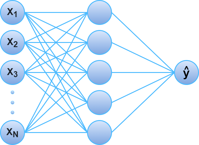
In the classic fully-connected feed-forward neural network, this structure of layers is ordered and connected such that every node $n_j$ in layer $L_i$ receives the output of every node in the preceding layer $L_{i-1}$, does some computation with those outputs, and passes the corresponding output to each node in the succeeding layer $L_{i + 1}$. The image above displays a neural network with $N$ input features, a single hidden layer, and a single output prediction $\hat{y}$.

Each node in layer $L_i$ contains some set of weights ($w$) and a bias ($b$), where the dimension of the weight vector is equal to the number of nodes in layer $L_{i - 1}$. When the node receives the output of all the nodes in the preceding layer, it performs the following computation: $L_{i - 1}^Tw + b$.

This should look familiar! It is quite literally $X^T\beta$: the classic computation from linear models on the outputs of the preceding layer!

However, before this node passes $X^T\beta$ to the next layer in the network, it is passed through an activation function $f$. Activation functions often introduce non-linearity to the NN, similar to link functions in GLMs. This non-linearity is important to increase the expressive power of the network. The composition of two linear functions is also linear. Because the computation on the node in a NN is the same as linear models, passing that to a non-linear activation function is necessary to expand the space of functions we can learn to span all continous functions.

The image below isolates a single neuron from the image above, taking input from the previous layer, and making a prediction by transforming the output of the neuron with an activation function $\hat{y} = f(X^T\beta)$.

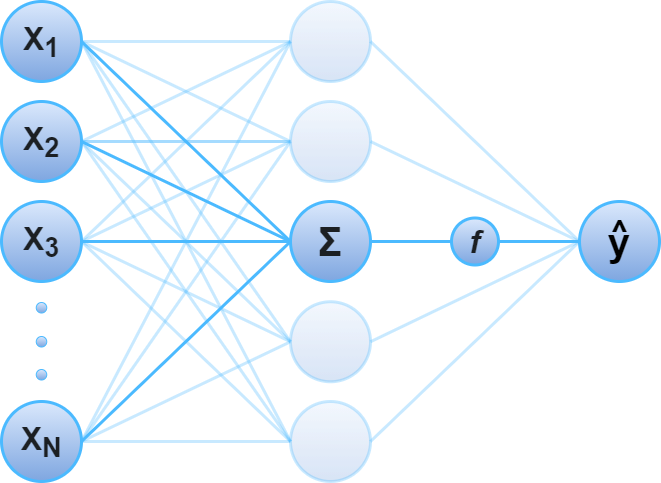
In fact, observe that if the activation function is invertible, this computation is equivalent to $f^{-1}(\hat{y}) = X^T\beta$, which is exactly a GLM with link function $f^{-1}$. This demonstrates that the computation of a single node in a neural network is, conceptually, a GLM on the output of the previous layer!

Furthermore, this means that a neural network with zero hidden layers and a linear activation function on the output layer is exactly equivalent to linear regression, as the lack of hidden layers maintains independence. And, if we change the activation function to the inverse of the logit function (this is the sigmoid activation function), this neural network becomes exactly equivalent to logistic regression! The code below is a simple prototype of building linear and logistic regression with PyTorch, and tests it on a simulated dataset.

import torch
import torch.nn as nn

class LinearRegression(nn.Module):
    def __init__(self, n_features):
        super().__init__()
        # zero hidden layers with a linear output
        self.output_layer = nn.Linear(n_features, 1)

    def forward(self, x):
        return self.output_layer(x)

class LogisticRegression(nn.Module):
    def __init__(self, n_features):
        super().__init__()
        # zero hidden layers with a sigmoid activation on one output node
        self.output_layer = nn.Linear(n_features, 1)

    def forward(self, x):
        return torch.sigmoid(self.output_layer(x))

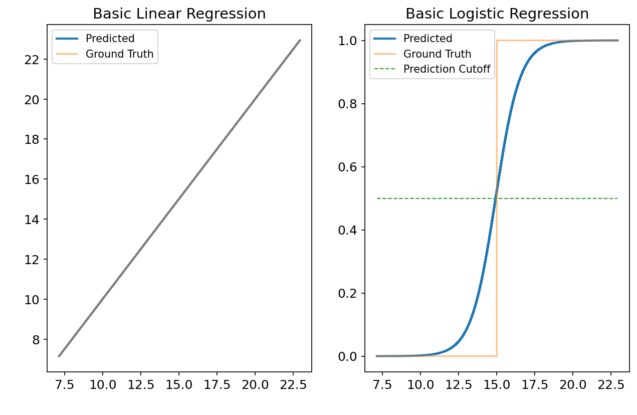
Hopefully if the math wasn’t convincing enough, these plots convince you that our neural network with a single input layer, zero hidden layers, and a single output node with a linear/sigmoid activation function is mathematically equivalent to linear/logistic regression.

Now that you have an understanding of all the components of neural networks with respect to linear models, the last piece to understand is the hidden layers.

Understanding Hidden Layers

As described in the previous section, hidden layers are the layers between the input and the output layer. They often have an activation function, which introduces non-linearity to the function we fit. Furthermore, introducing hidden layers are what is responsible for the opacity of neural networks. It’s why they are referred to as “black boxes”, meaning they are difficult to interpret.

This opacity doesn’t actually come from the non-linearity, but rather feature interactions. Because the nodes in a neural network compute the sum of the output of the nodes in the previous layer, once a single hidden layer is introduced, every node after the first hidden layer is computing a function that is dependent on every single input feature. This makes it difficult to see the individual contribution of a single input feature on the output of the network. The image below isolates the computation of single a node in a hidden layer between other hidden layers.

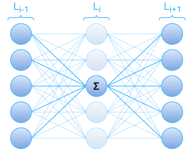
Let’s look at the math for regression using a neural network with $k$ hidden layers, where $w_{i,j}$ and $b_{i,j}$ are the weights and bias of the j^th node in layer $L_i$ with activation function $f_i$. As additional context, with the notation below, $f_i(L_{i - 1}^Tw_{i,3} + b_{i,3})$ corresponds to the computation of the highlighted node in the image above: the third node in the i^th layer.

$$\begin{aligned} L_0& = \big [ X_1, X_2, \cdots, X_n \big ] \\ L_1 & = \big [\hspace{0.5em}f_1(L_0^Tw_{1,1} + b_{1,1}), \hspace{0.5em}f_1(L_0^Tw_{1,2} + b_{1,2}), \cdots \big ] \\ & \vdots \\ L_k & = \big [\hspace{0.5em}f_k(L_{k - 1}^Tw_{k,1} + b_{k,1}), \hspace{0.5em}f_k(L_{k - 1}^Tw_{k,2} + b_{k,2}), \cdots \big ] \\ \hat{y} & = L_k^T \beta \end{aligned}$$

When you think of a hidden layer, think of it as a collection of models. Hidden layer $L_k$ in the math above is kind of like a list of Generalized Linear Models. The first element in $L_k$ is $f_k(L_{k - 1}^Tw_{k,1} + b_{k,1})$, which is basically like a GLM with link function $f_k^{-1}$ where the input features are the vector $L_{k - 1}$, the outputs of the nodes in the preceding layer. However, the analogy to GLMs is not perfect for a few reasons. First, The elements in $L_{k - 1}$ are not independent because they all are linear combinations of the input features. And second, activation function $f_k$ isn’t always invertible (e.g. ReLU. The point I am trying to make is that the math is familiar, as it’s intimately related to that of GLMs.

So why does this work so well? What is the intuition behind it?

Look at the last line in the equation above. The ouput prediction: $\hat{y} = L_k^T \beta$. If we think of $L_k$ as a collection of non-linear models dependent on every input feature as I described above, then we can also think of the output of each model in $L_k$ as an engineered feature. The purpose of hidden layers is basically automated feature engineering. The last hidden layer contains a bunch of engineered features that come from adding up a bunch of linear combinations of the input features and applying non-linear activation functions. These engineered features are then thrown into a linear model to predict the target.

So, neural networks really aren’t that different from linear models. They’re just instructions for learning the best features one can engineer from the input features, and predicting a linear combination of the engineered features!

Further Reading

Hopefully this blog post helped you understand how neural networks work! However, there is quite a lot that I didn’t cover. Below is a list of introductory resources on concepts related to neural networks that I didn’t cover:

1. Architecture: I only covered what classic fully connected feed forward neural networks look like in this blog post. There are a huge number of distinct types of neural networks, and which is best is quite dependent on application needs. This post provides diagrams and descriptions for almost 30 different neural architectures.
2. Activation Functions: Selecting the activation functions for introducing non-linearity into your neural network requires building up some intuition on how they work and how they impact learning. This post provides a nice overview of many activation functions as well as an introduction to the intuition and math behind when to use which activation function.
3. Optimization: These algorithms determine how a neural network learns the weights and biases. Most variants of optimization algorithms you will come across are some form of gradient descent. This post covers different variations of gradient descent optimization algorithms, and this post covers some additional optimization methods. Finally, this post covers backpropogation, which is the algorithm that computes the gradients necessary for all of the optimization algorithms in the other linked blog posts.
4. Regularization: Regularization is a technique that adds a penalty to the loss function in order to prevent overfitting and help machine learning algorithms generalize. This post provides a variety of example problems for regularization and introduces a variety of different regularization techniques.

---

References

1. Hornik, Stinchcombe & White, “Multilayer feedforward networks are universal approximators”, Neural Networks, 1989. ↩
2. Nelder & Wedderburn, “Generalized Linear Models”, Journal of the Royal Statistical Society, 1972. ↩

---

Footnotes

1. This means that there does not exist a set of scalars $[\alpha_1,\alpha_2,\cdots,\alpha_n]$, where at least one such $\alpha$ is non-zero, such that $\alpha_1 X_1 + \alpha_2 X_2 + \cdots + \alpha_n X_n = 0$. In other words, there is no multi-colinearity in $X$ and that the rows of $X$ must span the columns. ↩

2. The closed form solution for OLS is $\beta = (X^TX)^{-1} X^Ty$. This requires $X^TX$ to be invertible, which is the case when the elements in $X$ are linearly independent. This is satisfied by our assumption of independence. Without this assumption, there is no closed form solution, and $\beta$ can be approximated by the maximum likelihood estimation function: $min_\beta(y - \beta X)^T(y - \beta X)$. ↩

3. The exponential family is a particular family of probability distributions such that their probability density function (PDF) can be writted as: $P(x | \theta) = f(x) g(\theta) exp \Big( \eta(\theta) \cdot T(x) \Big)$, where $f$, $g$, $\eta$, and $T$ are known functions and $\theta \in \mathbb{R}$ is the only parameter to the PDF. ↩