Designing Transparent Neural Networks


Most systems we interact with are part of some pipeline that integrates Machine Learning (ML). Sometimes we interact with an ML model directly, like Spotify's recommender system for songs. Other times, this interaction is more detatched; we post a comment on Twitter or Facebook, and this comment is used to train some language model at the respective company. As ML models become more and more prevalent, interpreting and explaining the decisions these models make become increasingly important.
Neural networks (NNs) are a popular class of machine learning algorithms, which are notorious for being difficult to interpret. They are often referred to as "black boxes" or "opaque". Linear Models, Generalized Linear Models (GLMs), and Generalized Additive Models (GAMs) are examples of popular machine learning algorithms that are not "opaque", but instead "transparent". This transparency often leads linear and additive models to be favorable choices over classic neural networks even though the functions neural networks can learn are a superset of the functions these other models can learn. The goal of this blog post is to demonstrate that, with a particular asterix over the architecture of neural networks, they can be just as transparent.
![]()
Prior to jumping into such a neural architecture, it's important to understand the fundamental transparent algorithms. The following section will provide a quick background on the math and fundamentals for Generalized Additive Models, which is what will inspire our neural architecture design. GAMs are a special kind of GLM, and if you are not familiar with GLMs and how they are connected to Neural Networks, I would recommend reading the blog post below before reading this one:
Generalized Additive Models
Generalized Additive Models (GAMs), introduced in (Hastie & Tibshirani, 1986), take another step towards reducing the restrictions within linear models. There are two modifications that GAMs make to classic GLMs, which truly moves from rigid assumptions to flexible modeling:
-
Allow non-linearity: GAMs wrap each component $X_i$ with a function $h_k$, where $h_k$ is some learned function that can be non-linear, but must be smooth1. It is also usually non-parametric.
-
Feature interaction: The systematic component can be an equation that contains non-linear feature interaction like $h_k(X_i,X_j, \cdots)$.
Hence, equations for GAMs could look like this:
$$g(\mu(X)) = \beta_0 + h_1(X_1) + h_2(X_2, X_3) + \cdots + h_m(X_n) + \epsilon$$
Technically, this makes GLMs a special case of GAMs where all functions $h_k$ simply multiply their corresponding input feature(s) by a single parameter $\beta_k$. However, unlike GLMs, these functions require a more convoluted fitting mechanism. If you are interested in the history of GAMs and how they are fit, please refer to the original papers on the backfitting algorithm: (Friedman & Stuetzle, 1981), (Breiman & Friedman, 1985).
Don't worry if you are not familiar with some of the terms (e.g. b-spline), as they won't be relevant to the main body of this blog post about transparent neural networks. What follows is a simplification to provide intuition on what these $h_k$ functions are.
$$h_k(x_i) = \sum_{j=1}^n b_j(x_i)\beta_j$$
Where $b_j$ is a b-spline, $\beta_j$ is a learned coefficient corresponding to $b_j$, and $n$ is a hyperparameter describing the number of b-splines to use to fit the GAM. A linear combination of b-splines uniquely describes any spline function sharing the same properties as the b-splines (Prautzsch et al., 2002), which means these $h_k$ functions are spline functions. Below is an example of fitting a smooth function ($h_k(x_i) = sin(x_i)$) using a linear combination of b-splines.

As you can see, a linear combination of many cubic b-splines was sufficient to fit this smooth function. GAMs try and fit spline functions to transform each individual dependent variable, and model the independent variable as a linear combination of these spline functions. This maintains transparency because, once fit, we can inspect the learned functions to understand exactly how our model makes predictions according to individual features.
There is so much more to learn about GAMs, such as how these splines are learned, methods of interpreting them, and important regularization penalties to ensure higher degrees of smoothness. There are even some newer methods of fitting GAMs using decision trees instead of splines. If you would like a more extensive review on GAMs, please refer to this wonderful mini-website-textbook, however that's out of the scope of this blog post.
Transparent Neural Networks
(Hornik et al., 1989) is the original paper suggesting NNs are a type of universal approximator. The theory of this contribution was explored in multi-layer perceptrons in (Pinkus, 1999) and generally formalized by (Balázs, 2001). The theorem can be summarized by:
A neural network with a single hidden layer of infinite width can approximate any continuous function.
If neural networks can be used to approximate any continuous function, then they can be used to approximate the non-linear, non-parametric, functions ($h_k$ in the previous section) necessary for Generalized Additive Models. Furthermore, neural networks can describe a wider set of functions than GAMs because continuous functions don't have to be smooth, while smooth functions have to be continuous.

Above are images of three functions. The first function is a linear combination of the second and third function2. Observe that all three functions are continuous. We would like to build a model that can fit the first function, while maintaining feature-wise interpretability such that we can see that it properly learns the second and third functions. Unfortunately, it is not reasonable to expect a GAM to achieve this because, while the functions are continuous, they are not smooth. Below is a GAM with very low regularization and smoothness penalties in order to let it try and fit non-smooth functions. Furthermore, it is trained and tested on the same dataset. This is a strong demonstration that GAMs cannot approach these problems, because they can't even overfit to the solution.
from pygam import LinearGAM
from pygam import s as spline
#fit a classic GAM with no regularization or smoothing penalties to try and
#let it overfit to non-smooth functions. It still fails!
gam = LinearGAM(
    spline(0,lam=0,penalties=None) +
    spline(1,lam=0,penalties=None),
    callbacks=[]
).fit(X, y)

While these fits aren't terrible in terms of prediction error, that's not what we care about. We care about learning the proper structure for the functions that explain the relationship between individual features and our output. The above plots are a clear demonstration that GAMs can't even overfit to provide that.
Luckily, because these functions are continuous, we can use a neural network to approximate them!
Generalized Additive Neural Networks
The trick is to use a different neural network for each individual feature, and add them together just like how GAMs work! By replacing the non-linear, non-parametric, functions in GAMs by neural networks, we get Generalized Additive Neural Networks (GANNs), introduced in (Potts, 1999). Unfortunately, this contribution did not take off because we didn't have the technical capacity to train large networks as we do today. Luckily, now it is quite easy to fit such a model.
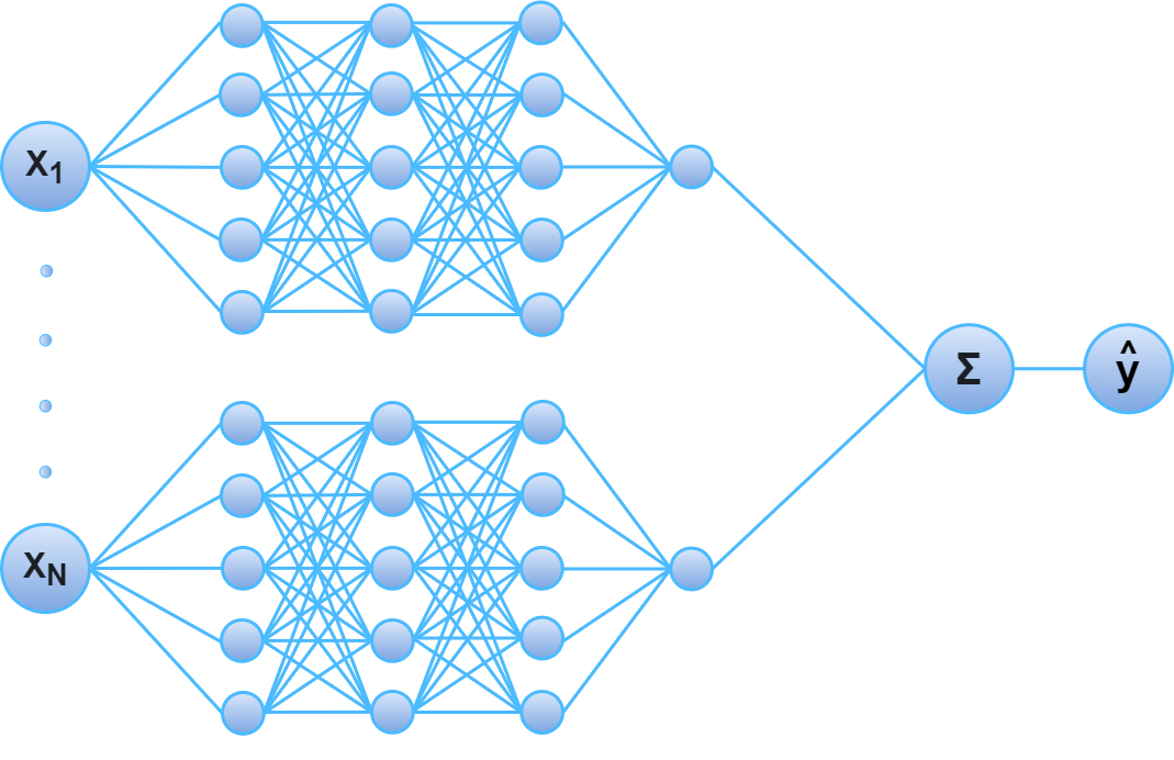
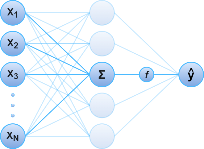
GANNs are simply a linear combination of neural networks, where each network only observes a single input feature3. Because each of these networks take a single input feature, and provide a single output feature, it becomes possible to plot a two-dimensional graph where the x-axis is the input feature and the y-axis is the output feature for each network. This graph is hence a fully transparent function describing how the neural network learned to transform the input feature as it contributes, additively, to the prediction. Hence this type of neural architecture is sufficient for creating a model as transparent as classic linear and additive models described in this blog post so far.
Below is code for creating a GANN using Keras. As you can see, this model is capable of solving the regression problem while maintaining feature-wise transparency on piecewise continous functions!
import tensorflow as tf
from tensorflow.keras import layers, Model

#define a simple multi-layer perceptron
class NN(Model):
    def __init__(
        self,
        name=None
    ):
        super().__init__(name=name)
        # relu helps learn more jagged functions if necessary.
        self.l1 = layers.Dense(8, activation='relu')
        # softplus helps smooth between the jagged areas from above
        #     as softplus is referred to as "SmoothRELU"
        self.l2 = layers.Dense(8, activation='softplus')
        self.l3 = layers.Dense(8, activation='softplus')
        self.l4 = layers.Dense(8, activation='softplus')
        self.output_layer = layers.Dense(1)

    def call(self, x, training=None):
        x = self.l1(x)
        x = self.l2(x)
        x = self.l3(x)
        x = self.l4(x)
        return self.output_layer(x)

#define a Generalized Additive Neural Network for n features
class GANN(Model):
    def __init__(
        self,
        n_features,
        name=None
    ):
        super().__init__(name=name)
        self.n_features = n_features
        # initialize MLP for each input feature
        self.components = [NN() for i in range(n_features)]
        # create final layer for a linear combination of learned components
        self.linear_combination = layers.Dense(1)

    @tf.function
    def call(self, x, training=None):
        #split up by individual features
        individual_features = tf.split(x, self.n_features, axis=1)
        components = []
        #apply the proper MLP to each individual feature
        for f_idx,individual_feature in enumerate(individual_features):
            component = self.components[f_idx](individual_feature)
            components.append(component)
        #concatenate learned components and return linear combination of them
        components = tf.concat(components, axis=1)
        return self.linear_combination(components)
model = GANN(n_features=2)
model.compile(
    optimizer=tf.keras.optimizers.Adam(),
    loss='mean_squared_error',
    metrics=['mean_absolute_error']
)
hist = model.fit(
    X.to_numpy(),
    y.to_numpy(),
    epochs=50,
    batch_size=32,
)

At first glance, these results look good, but not perfect. The first plot demonstrates this model achieved a near perfect fit of the actual task, while the last two plots look like the GANN was capable of learning the general shapes of the functions, but is off on the intercepts for all of them. This should not discount the validity of the model. The corresponding math demonstrates perfectly fitting intercepts of an additive model cannot be guaranteed.
Let $h_i(X_i) = \alpha_i + f(X_i)$ where $f(X_i)$ represents all of the aspects of $h(X_i)$ that dependent on $X_i$, and $\alpha_i$ represents the intercept.
$$ \begin{aligned} y & = \beta_0 + \sum_{i=1}^n \beta_i h_i(X_i) \\ & = \beta_0 + \sum_{i=1}^n \beta_i (\alpha_i + f_i(X_i)) \\ & = \beta_0 + \sum_{i=1}^n \beta_i \alpha_i + \sum_{i=1}^n \beta_i f_i(X_i) \end{aligned} $$The only way to tease apart these intercepts is via $\beta$. Imagine the proper fit of this equation, for every $i$, had $\beta_i = 1$ and $\alpha_i = 2$. In this case, if half of the learned $\alpha_i$s are zero, and the other half are four, that would yield the exact same result for $\sum_{i=1}^n \beta_i \alpha_i$ as the proper fit. Hence, by way of contradictory example, it is impossible to guarantee learning correct intercepts for the individual components of any additive model.
The plots below are what happens when we simply adjust the learned intercepts for these functions. As you can see, by simply changing the intercept, we are able to show a near perfect fit of these functions, which is the best we can ever hope to do! Furthermore, we can explore the derivatives of these functions to measure the goodness of fit because the rate of change of the function is entirely independent of the intercept.


This is a clear demonstration that Generalized Additive Neural Networks are capable of overfitting to piecewise continuous functions while maintaining transparency!
The next section provides a brief overview of Neural Additive Models (NAMs), which are a special variant of GANNs that are designed to be able to fit "jumpy functions", as this is more reminiscient of real-world data.
Neural Additive Models
Real world data doesn't look like beautifully continuous functions. It's often messy, and there will be multiple data points with extremely similar features that have noticeably different results. Many machine learning models have existing structure that prevents learning functions that look crazy and jump all over the place. Linear regression has to learn the best fitting line because $X^T\beta$ can't describe a "jumpy" function. GAMs are regularized to enforce smoothness to prevent this as well. (Agarwal et al., 2020) explores a particular modification to the mathematic computations made on nodes in GANNs in order to let them fit "jumpy" functions. They call these modified nodes "exp-centered hidden units" or "ExU units", and they work as follows:
Let $w$ and $b$ be the respective weight and bias parameters on a node with activation function $f$. Then, when the node is passed input $x$ it computes: $f(e^w * (x - b))$. Recall that the normal computation on these nodes is simply applying the activation function to a linear computation: $f(w * x + b)$. The reason exponentiation of the weights accomplishes the goal of learning "jumpy" functions is that small changes in the input can have drastic changes on the output, enabling small weights to still represent a function with a steep slope. The excerpt below is taken directly from (Agarwal et al., 2020) and demonstrates the difference between a non-regularized neural network's ability to overfit to data when using normal node computation (a) versus ExU unit computation (b).
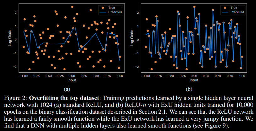
While this clearly demonstrates ExU's ability to overfit to jumpy functions, this isn't ideal. Overfitting isn't a good thing. Hence, the rest of this paper demonstrates ExU can be regularized to learn functions that are relatively smooth, yet "jumpy" at very specific junctions. This is more reminiscient of real-world solutions, and the paper shows that this can outperform current state-of-the-art GAMs while maintaining feature transparency. Their regularization strategies are:
- Dropout: randomly zero-out nodes inside each NN.
- Weight Decay: add a penalty corresponding to the L2 norm of weights inside each NN.
- Output Penalty: add a penalty corresponding to the L2 norm of the outputs of each NN.
- Feature Dropout: randomly exclude entire features from the NAM.
ExU and these regularization techniques are the only difference between NAMs and GANNs, and it fundamentally changes the loss landscape in a way that enables learning "jumpy" functions. GANNs are a very general architectural description, and there are many perturbations on the architecture, such as NAMs, that can make them well suited for your problem. The final section in this blog post will discuss the computational graph, and how to leverage understanding a specific problem to design a transparent neural network.
Designing Your Computational Graph
Hopefully the review of the NAM paper motivated some curiosity and creativity. The nodes and feature-networks in GANNs don't need to be the classic feed-forward-neural-network you may be familiar with. Furthermore, there is no reason all of these feature-networks have to be the same. They can have different numbers of layers, different activation functions, and different architectures all together.
A neural network can be described as a computational graph. It's a graph that describes a directed order of computation in order to go from some input to some output. The general description of the order of computations of a GANN is:
- Define a finite set of modules (NNs), and specify which features go into which modules.
- Make your prediction as a linear combination of the output of these modules.
The second point is what makes the model a GANN. It's what specifies the model as strictly additive. We can make a slight modification to this description to further generalize into transparent models that are not strictly additive.
- Define a finite set of modules, and specify which features go into which modules.
- Define a function that specifies how the outputs of each module are used for prediction.
The second point here is more general than that of a GANN, because "a linear combination of the output of these modules" is one such example of "a function that specifies how the outputs of each module are used". As this blog post has demonstrated, transparency is all about control of the input features. That last operation that is a linear combination of all these feature-neural-networks doesn't have to be how they are used! Based on an expert understanding of your data and your problem, you can define a function you would like to fit. And, as long as you code up a computational graph that doesn't entangle all the features in opaque ways, you can fit that function with a collection of neural networks just like how GANNs work!
Let's walk through a simple example:
Let's say you have 5 features $[x_1, x_2, x_3, x_4, x_5]$. And let's say that you believe, according to features $x_1$ and $x_2$, the solution to your problem should treat the other features differently. We can describe our equation as follows:
Let $f_1(x_1, x_2) \in \{0,1\}$
Let $f_2(x_3, x_4, x_5) \in \Reals$
Let $f_3(x_3, x_4, x_5) \in \Reals$
Then, we want to solve:
$$ \hat{y} = (f_1(x_1, x_2)) * f_2(x_3, x_4, x_5) + (1 - f_1(x_1, x_2)) * f_3(x_3, x_4, x_5) $$Specifically, the purpose of $f_1$ is to learn some binary feature to determine how the model handles the other features. if $f_1(x_1, x_2) = 0$, then the model will use $f_3$, otherwise it will use $f_2$. You can solve this problem with three neural networks, one for each function. Then, rather than having the prediction be a normal linear combination of those three functions like a GANN, you set the prediction to correspond to the equation above.
I have simulated a dataset that defines $f_1$ as whether $x_1,x_2$ are inside the unit circle, and defines $f_2$ and $f_3$ as basic linear models4. The code below defines a a neural network that learns these three functions to make a prediction. And below I show the results to demonstrate that we learn the correct circle boundaries and linear models, which maintains full transparency!
Additional Note: this specific example requires learning a conditional function $f_1$, which is not continuous and hence requires some tricks to learn via neural networks. You can see my code below for the BinaryNN, which learns a continuous function, modifies it to be binary, but applies backpropigation as if that modification was the identity function. This is called the Straight-Through estimator, and was introduced by Hinton in his 2012 Coursera lectures. Refer to (Bengio et al., 2013) If you'd like further reading on conditional computation.
class BinaryNN(Model):
    def __init__(
        self,
        threshold=0.5,
        name=None
    ):
        super().__init__(name=name)
        self.threshold = threshold
        self.l1 = layers.Dense(8, activation='relu')
        self.l2 = layers.Dense(8, activation='relu')
        self.l3 = layers.Dense(8, activation='relu')
        #sigmoid to ensure the output is in the range 0,1
        # before we round to be binary
        self.output_layer = layers.Dense(1, activation='sigmoid')

    def call(self, x, training=None):
        x = self.l1(x)
        x = self.l2(x)
        x = self.l3(x)
        x = self.output_layer(x)
        return self.round_to_binary(x)

    def round_to_binary(self, x):
        """
        x is a number between 0 and 1, and is set
            to be 0 if less than self.threshold, 1
            if greater than self.threshold.

        Computing the factor to add to x in order to
            round accordingly is not a differentiable
            operation, so we wrap it in tf.stop_gradient
            so that it is treated as a constant when
            differentiating.
        """
        return x + tf.stop_gradient(
            tf.cast(x > self.threshold, tf.float32) - x
        )
class TransparentNN(Model):
    def __init__(
        self,
        threshold=0.5,
        binary_idx=2,
    ):
        super().__init__()
        self.binary_idx = binary_idx
        #layer for learning a function that maps to a binary
        # label according to a specified threshold
        self.binary_layer = BinaryNN(threshold=threshold)
        #two different linear regression models where linear_1
        # is used when the binary layer specifies 1, otherwise
        # we use linear_2
        self.linear_1 = layers.Dense(1, activation="linear")
        self.linear_2 = layers.Dense(1, activation="linear")
        #note: if you want to model this as a complex non-linear
        # function, you can replace these dense layers with an MLP

    def call(self, input_layer, training=None):
        #get features to pass to the binary layer
        binary_slice = input_layer[:,:self.binary_idx]
        #get features to pass to the linear layers
        linear_slice = input_layer[:,self.binary_idx:]
        #compute binary flag
        binary_flag = self.binary_layer(binary_slice)
        #return the function we are trying to model
        return (
            (binary_flag) * self.linear_1(linear_slice) +
            (1 - binary_flag) * self.linear_2(linear_slice)
        )
model = TransparentNN(threshold=0.5)
model.compile(
    optimizer=tf.keras.optimizers.Adam(),
    loss='mean_squared_error',
    metrics=['mean_absolute_error']
)
hist = model.fit(
    x,
    y,
    epochs=50,
    batch_size=32,
)

As you can see above, our neural network designed to fit our specified function was properly able to learn both weights of the linear models and the circular boundary to determine which linear model to use and is hence interpretable.
This whole blog post built up to an understanding of how additive models can maintain feature-wise interpretability, and that it's possible to design a neural network architecture that leverages that. However, the computational graph generalizes even further, and I hope the example above helped demonstrate that. Focus on the math. Focus on the specifics of the problem at hand. You can design interpretable architectures as a function of these feature-networks as long as you meticulously control how the features interact according to the computational graph. Then, because you controlled and isolated features in the computational graph, you can easily discern how those features were used in order to make the final prediction $\hat{y}$, which is the definition of a transparent model!
- Hastie, T., & Tibshirani, R. (1986). Generalized Additive Models. Statist. Sci., 1(3), 297–310. https://doi.org/10.1214/ss/1177013604
- Friedman, J. H., & Stuetzle, W. (1981). Projection Pursuit Regression. Journal of the American Statistical Association, 76(376), 817–823. https://doi.org/10.1080/01621459.1981.10477729
- Breiman, L., & Friedman, J. H. (1985). Estimating Optimal Transformations for Multiple Regression and Correlation. Journal of the American Statistical Association, 80(391), 580–598. https://doi.org/10.1080/01621459.1985.10478157
- Prautzsch, H., Boehm, W., & Paluszny, M. (2002). Bézier and B-Spline Techniques. https://doi.org/10.1007/978-3-662-04919-8
- Hornik, K., Stinchcombe, M., & White, H. (1989). Multilayer feedforward networks are universal approximators. Neural Networks, 2(5), 359–366. https://doi.org/https://doi.org/10.1016/0893-6080(89)90020-8
- Pinkus, A. (1999). Approximation theory of the MLP model in neural networks. Acta Numerica, 8, 143–195. https://doi.org/10.1017/S0962492900002919
- Balázs, C. (2001). Approximation with Artificial Neural Networks. https://doi.org/10.1.1.101.2647
- Potts, W. J. E. (1999). Generalized Additive Neural Networks. Proceedings of the Fifth ACM SIGKDD International Conference on Knowledge Discovery and Data Mining, 194–200. https://doi.org/10.1145/312129.312228
- Agarwal, R., Frosst, N., Zhang, X., Caruana, R., & Hinton, G. E. (2020). Neural Additive Models: Interpretable Machine Learning with Neural Nets.
- Bengio, Y., Léonard, N., & Courville, A. C. (2013). Estimating or Propagating Gradients Through Stochastic Neurons for Conditional Computation. CoRR, abs/1308.3432. http://arxiv.org/abs/1308.3432
- The "smoothness" of a function is described by the continuity of the derivatives. The set of functions with a smoothness of 0 is equivalent to the set of continuous functions. The set of functions with a smoothness of 1 is the set of continuous functions such that their first derivative is continuous. So on, and so forth. Generally, a function is considered "smooth" if it has "smoothness" of $\infty$. In other words, it is infinitely differentiable.↩
- The actual function being fit here is $f(x_1,x_2) = a(x_1) + b(x_2)$, however I plot the function $f(x_1 + x_2) = a(x_1) + b(x_2)$ in order to project it as two-dimensional, as that is easier for readers to look at.↩
- Technically, this could be fit where the sub-networks take more than a single feature as input, but this comes at a cost of interpretability. It is still possible to explore the relationship between both features and the output, however it becomes high-dimensional, entangled, and hence more difficult to interpret.↩
- I am setting $f_2$ and $f_3$ as linear models for simplicity in demonstrating a transparent model. This methodology ports over to any function you would want to define as $f_2$ and $f_3$.↩